An iterative exploration on EM algorithm

January 2, 2024

An iterative exploration on EM algorithm #

As a continuation of my notes on classicial machine learning, this is an exclusive study on EM agorithm to deepen my understanding from a wider variety of perspectives.

EM as Expection + Maximization #

The understanding of latent variable is the first `get` in EM algorithms.

Through latent variable, we have witnessed the greatness of EM algorithm which breaks through the limit of MLE.

Likelihood of latent variables:

E-step:

M-step:

Here’s the same example using a Gaussian Mixture Model (GMM) with two components in Python, using NumPy and SciPy:

1. Import required libraries and generate data:

import numpy as np
from scipy.stats import norm

np.random.seed(42)
data = np.concatenate((np.random.normal(1, 1, 100), np.random.normal(5, 1, 100)))

print(len(data))
print(data[:5])

2. Define the log-likelihood function for the complete data (X, Z):

def log_likelihood(data, means, pis, k):
    return np.sum(np.log(np.sum(pis[j] * norm.pdf(data, means[j], 1) for j in range(k))))

3. Implement the EM algorithm:

def EM(data, k, max_iterations):
    means = np.random.uniform(np.min(data), np.max(data), k)
    pis = np.full(k, 1/k)

    for _ in range(max_iterations):
        # E-step
        assignments = np.array([[pis[j] * norm.pdf(x, means[j], 1) for j in range(k)] for x in data])
        assignments = assignments / np.sum(assignments, axis=1).reshape(-1, 1)

        # M-step
        means = np.sum(assignments * data.reshape(-1, 1), axis=0) / np.sum(assignments, axis=0)
        pis = np.sum(assignments, axis=0) / len(data)

    return means, pis

4. Run the EM algorithm with the generated data, 2 components, and 50 iterations:

means, pis = EM(data, 2, 50)

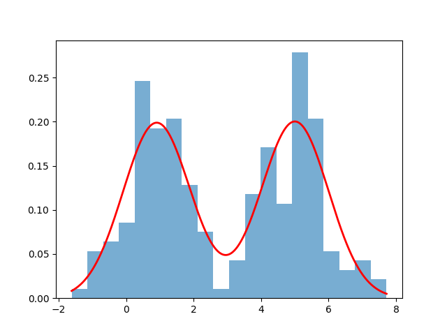
5. Visualize the result:

import matplotlib.pyplot as plt

plt.hist(data, bins=20, density=True, alpha=0.6)
x = np.linspace(np.min(data), np.max(data), 1000)
gmm_pdf = pis[0] * norm.pdf(x, means[0], 1) + pis[1] * norm.pdf(x, means[1], 1)
plt.plot(x, gmm_pdf, 'r-', linewidth=2)
plt.savefig("./gmm_pdf.png")
plt.show()

EM as a local lower bound construction #

If you delve deeper into the convergence proof of the EM algorithm based on latent variables, using the Jensen’s inequality construction for the log(x) function ¹, we can easily prove that the EM algorithm repeatedly constructs new lower bounds and then further solves them.

Thus the EM process can be seen as: fix the current parameters \(\theta_n\) first, calculate a lower bound function for the distribution of the latent variables, optimize this function to obtain new parameters, and then repeat.

The EM process described here is connected to the Variational Bayes (VB) method:

Variational Bayes can be seen as an extension of the expectation-maximization (EM) algorithm from maximum a posteriori estimation (MAP estimation) of the single most probable value of each parameter to fully Bayesian estimation which computes (an approximation to) the entire posterior distribution of the parameters and latent variables. As in EM, it finds a set of optimal parameter values, and it has the same alternating structure as does EM, based on a set of interlocked (mutually dependent) equations that cannot be solved analytically.

Both methods involve finding approximate solutions to intractable optimization problems by constructing lower bounds for the objective functions. Similarly, in the Variational Bayes method, the goal is to approximate the posterior distribution of latent variables by minimizing the Kullback-Leibler (KL) divergence between the true posterior distribution and the approximate distribution. This is achieved by constructing a lower-bound function for the log marginal likelihood, called the Evidence Lower Bound (ELBO), and optimizing this lower-bound function with respect to the approximate distribution.

K-means as a hard EM #

Based on the understanding of the second level, you can now freely apply the EM algorithm to GMM and HMM models. Especially after a deep understanding of GMM, for the joint probability with latent variables, when using the Gaussian distribution as a substitute:

This formula represents the joint probability distribution for a set of observed variables \(x_1, \ldots, x_n\) and latent variables \(z_1, \ldots, z_n\) under a Gaussian Mixture Model (GMM) with parameter \(\Theta\) .

The formula can be broken down as follows:

1. \(P_{\Theta}\left(x_1, \ldots, x_n, z_1, \ldots z_n\right)\) : This is the joint probability of the observed variables \(x_1, \ldots, x_n\) and the latent variables \(z_1, \ldots, z_n\) under parameter \(\Theta\) .
2. \(\prod_{t=1}^N P_{\Theta}\left(z_t\right) P_{\Theta}\left(x_t \mid z_t\right)\) : This expression is the product of the prior probabilities of the latent variables \(z_t\) and the conditional probabilities of the observed variables \(x_t\) given the latent variables \(z_t\) . The product is taken over all \(N\) data points.
3. \(\frac{1}{K}\) : This term represents the uniform prior distribution of the latent variables \(z_t\) , where \(K\) is the number of Gaussian components in the GMM.
4. \(\mathcal{N}\left(\mu^{z_t}, I\right)\left(x_t\right)\) : This term is the conditional probability of the observed variable \(x_t\) given the latent variable \(z_t\) . It is modeled as a Gaussian distribution with mean \(\mu^{z_t}\) and identity covariance matrix \(I\) .

Easy to see a connection with MSE:

This formula represents the optimization problem for finding the optimal means \(\left(\mu^1, \ldots, \mu^K\right)^*\) of a Gaussian Mixture Model (GMM) by minimizing the mean squared distance between the data points and their corresponding means.

The formula can be broken down as follows:

1. \(\left(\mu^1, \ldots, \mu^K\right)^*\) : This represents the optimal means of the Gaussian components in the GMM.
2. \(\underset{\mu^1, \ldots, \mu^k}{\operatorname{argmin}}\) : This indicates that we are looking for the values of \(\mu^1, \ldots, \mu^k\) that minimize the expression that follows.
3. \(\underset{z_1, \ldots, z_n}{\min}\) : This indicates that we are looking for the values of the latent variables \(z_1, \ldots, z_n\) that minimize the expression that follows.
4. \(\sum\limits_{t=1}^N\left\|\mu^{z_t}-x_t\right\|^2\) : This is the sum of the squared Euclidean distances between each data point \(x_t\) and its corresponding mean \(\mu^{z_t}\) . The sum is taken over all \(N\) data points.

A simpler and more intuitive explanation is that the K-means algorithm uses a hard clustering algorithm, while the EM algorithm we are discussing is a soft clustering algorithm. The so-called hard is a binary decision, either it is or it isn’t (0-1 choice). On the other hand, the soft deals with situations like a data point always belongs to multiple clusters, and that a probability is calculated for each combination of data point and cluster.

This can be summarized as:

There is no “k-means algorithm”. There is MacQueens algorithm for k-means, the Lloyd/Forgy algorithm for k-means, the Hartigan-Wong method, …

There also isn’t “the” EM-algorithm. It is a general scheme of repeatedly expecting the likelihoods and then maximizing the model. The most popular variant of EM is also known as “Gaussian Mixture Modeling” (GMM), where the model are multivariate Gaussian distributions.

One can consider Lloyds algorithm to consist of two steps:

• the E-step, where each object is assigned to the centroid such that it is assigned to the most likely cluster.
• the M-step, where the model (centroids) are recomputed (least squares optimization).

… iterating these two steps, as done by Lloyd, makes this effectively an instance of the general EM scheme. It differs from GMM that:

• it uses hard partitioning, i.e. each object is assigned to exactly one cluster
• the model are centroids only, no covariances or variances are taken into account

EM as a special case of generalized EM #

We define the right side of Jensen’s inequality as the free energy.

This formula represents the free energy \(\mathcal{F}(q, \theta)\) , which is an important concept in variational inference and is used to approximate the log marginal likelihood. The formula consists of two parts:

1. \(\langle\log P(\mathcal{X}, \mathcal{Y} \mid \theta)\rangle_{q(\mathcal{X})}\) : This term represents the expected log joint probability of the observed data \(\mathcal{Y}\) and the latent variables \(\mathcal{X}\) given the model parameters \(\theta\) . The expectation is taken with respect to the approximate posterior distribution \(q(\mathcal{X})\) . This term measures the goodness-of-fit of the model to the data, taking into account the uncertainty in the latent variables.

2. \(\mathbf{H}[q]\) : This term represents the entropy of the approximate posterior distribution \(q(\mathcal{X})\) . It measures the uncertainty in the latent variables given the observed data. High entropy corresponds to a more dispersed distribution, while low entropy corresponds to a more concentrated distribution.

The free energy combines these two terms, balancing the goodness-of-fit of the model with the uncertainty in the latent variables. In variational inference, the goal is to minimize the free energy with respect to both the approximate posterior distribution \(q(\mathcal{X})\) and the model parameters \(\theta\) . This minimization leads to an approximation of the true posterior distribution of the latent variables and provides a lower bound on the log marginal likelihood.

Thus, E-step is to optimize the latent (approximate posterior) distribution \(q(\mathcal{X})\) with fixed model parameters \(\theta\) , and the M-step is to optimize \(\theta\) with a fixed \(q(\mathcal{X})\) . This is the generalized EM algorithm.

E-Step :

M-step:

After understanding the generalized EM algorithm, we delve deeper into free energy and discover the relationship between free energy, likelihood, and KL divergence. When the model parameters are fixed, the only option is to optimize the KL divergence. In this case, the hidden distribution can only take the following form:

In the EM algorithm, this is directly given. Therefore, the EM algorithm is a naturally optimal hidden distribution case within the generalized EM algorithm. However, in many cases, the hidden distribution is not so easy to compute…

One example where the hidden distribution is not easy to compute arises in the context of topic models, such as Latent Dirichlet Allocation (LDA). In LDA, the goal is to learn the hidden topics that generate a collection of documents. The observed data are the words in each document, and the latent variables are the topic assignments for each word. The hidden distribution in this case is the posterior distribution of the topic assignments given the observed words and the model parameters (topic-word probabilities and document-topic probabilities).

Computing the exact hidden distribution in LDA is challenging because the posterior distribution involves a large number of topic assignments, which grow exponentially with the number of words and topics. This makes exact inference intractable for all but the smallest datasets and simplest models.

To overcome this difficulty, various approximate inference techniques are employed in practice to estimate the hidden distribution in LDA, such as:

1. Gibbs sampling: A Markov chain Monte Carlo (MCMC) method that generates samples from the posterior distribution by iteratively sampling topic assignments for each word in the documents.
2. Variational inference: A deterministic method that approximates the true posterior distribution with a simpler distribution (e.g., a factorized distribution) and minimizes the KL divergence between the true and approximate distributions.
3. Collapsed variational inference or collapsed Gibbs sampling: Techniques that integrate out some of the model parameters (e.g., topic-word probabilities) to simplify the inference problem and reduce the computational complexity.